Spike detection
Chunking
JRCLUST will chunk up large files and perform each of the following steps in sequence over each chunk. If you are using a GPU, the chunk size is determined from your available GPU memory. For consistency, 3/4 of the total GPU memory will be considered “available”. If you are not using a GPU, JRCLUST will try to determine the total amount of RAM available on your system and consider all of it to be available. JRCLUST will then take a fraction of that available memory and reserve it for processing. Large files are chunked to use as much of the available memory as possible.
Denoising
JRCLUST constructs an adaptive notch filter which cleans narrow-band noise peaks exceeding a threshold you supply threshold you supply.
(Set this parameter (fftThresh) to 0 to skip this step.)
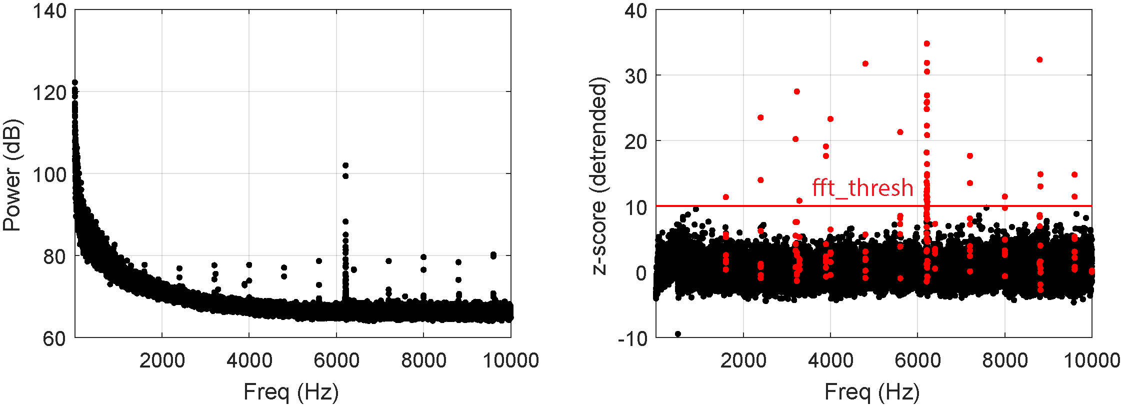
The time-domain signal is converted to the frequency domain via fast Fourier transform (FFT). After this, the average power across channels is computed. Power is (putatively) detrended using \(\frac 1 f\) relationship in frequency vs. power. For each frequency bin, the power-frequency product is normalized by its MAD, and those frequencies whose MAD power-frequency products exceed this threshold are zeroed out. The cleaned frequency-domain signal is then transformed back to the time domain via inverse FFT.
The figure below shows the original (left) and detrended (right) plots. Red indicates FFT coefficients that exceed threshold or points that are within 3 samples from the outlier points.
Filtering
This step filters the raw samples depending on the filter type you specify. Additionally, JRCLUST computes the common average reference and subtracts it from the filtered samples. (The meaning of “average” in “common average reference” is controlled by the CAR mode you specify.)
Computing detection thresholds
Assuming a Gaussian noise distribution on every site, we estimate the standard deviation \(\sigma_{\text{noise}}^{(i)}\) of the background on site \(i\) by
where \(x^{(i)}\) is the filtered signal on site \(i\). (See here for justification.) A single multiple of \(\sigma_{\text{noise}}^{(i)}\) that you specify serves as the detection threshold on each site. In other words, each site has a distinct threshold which is a multiple of an estimate of the standard deviation of its own noise distribution.
Detecting peaks
Samples on each site are compared to the threshold \(\text{Thr}_i\) for that site. Those samples with negative value but exceeding the threshold in magnitude are considered putative peaks. (If you specify, then JRCLUST can also detect peaks with positive value.) A putative peak must also exceed its immediate neighbors in magnitude, i.e., the sample at time \(t_j\) is a peak if and only if the following conditions hold:
You may also impose additional constraints on peak detection.
Merging peaks
Peak samples are compared with neighbors in a spatiotemporal window around each peak to detect duplicates. If peaks are found within this window, then the following operations are performed:
- If a neighboring peak has a larger amplitude, then discard the center peak.
- If a neighboring peak has the same amplitude but occurs first, then discard the center peak.
- If a neighboring peak has the same amplitude and occurs at the same time, then discard the peak occurring on the higher-indexed site.
Extract spatiotemporal windows around spiking events
For each spiking event, JRCLUST will save raw and filtered samples as \(n_{\text{sites}} \times n_{\text{samples}}\) matrices.
\(n_{\text{sites}}\) is nSitesEvt (determined from nSiteDir),
and \(n_{\text{samples}}\) depends on evtWindow and evtWindowRaw for filtered and raw samples, respectively.
Each of these matrices is stored in an \(n_{\text{sites}} \times n_{\text{samples}} \times n_{\text{spikes}}\)
array and are used for feature extraction, automatically merging clusters, and display in the curation GUI.
At this point, if you specify, JRCLUST may either subtract a local common average reference from the windows and realign the spike waveforms; or interpolate the spike waveforms between samples to determine if the true peak maxima are at subpixels, taking the interpolant if this is found to be the case.
Compute features from extracted waveforms
JRCLUST subtracts the local common-average reference from the spike waveforms extracted above and then computes features from these according to the feature you specify. For more detailed descriptions of your options in features, see below.
Additionally, if you specify, JRCLUST finds an alternate location for each spike within that spike’s spatiotemporal window. JRCLUST will extract a window around this secondary peak in order to compute features. This is done in order to accommodate necessary alterations to the clustering algorithm due to resource constraints.