Cluster curation

As a user, you will want to inspect your clusters as well as make corrections to the automatic detection and clustering done by JRCLUST. This is done via the manual curation GUI, which is invoked like so:

jrc manual /path/to/your/configfile.prm

This GUI allows you to annotate (i.e., add a note to), delete, or split clusters, as well as merge two clusters. To accomplish this, a number of figures are displayed. The figures to show are specified in the figList parameter, but it is recommended to leave this parameter alone. With any of the interactive figures, you may press the h key to display a small help dialog.

The waveform view (FigWav)

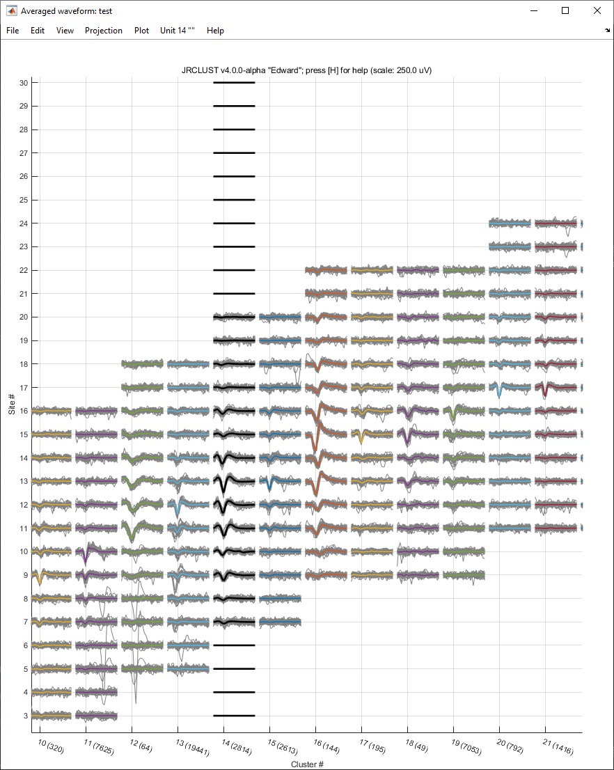
The waveform view is the main view on your data. Each cluster is ordered by its center site and the mean unit waveform is plotted for each site in a spatial neighborhood around the center. In the background, plotted in gray, are some randomly-sampled individual waveforms. (You can toggle these off and on by pressing the w key and resample them with the a key.) You can select clusters by clicking their waveforms. The selected cluster will be highlighted in black. Right-clicking another cluster will cause that cluster to be highlighted in red and update the other figures with data from each cluster for comparison. (Select the next most similar cluster by pressing the spacebar). You may pan by holding the Shift key and clicking and dragging, or zoom in and out with the scroll wheel. The left and right arrows will select the previous and next clusters, respectively. The up and down arrows adjust the scale of the waveforms. Pressing r will zoom out and show all clusters, while pressing z will zoom in on the selected cluster. If you have a trial file, pressing p will plot the peristimulus time histogram of the selected cluster. To delete the selected cluster, press d. To split the selected cluster, press s. To merge the selected pair of clusters, press m.

The waveform view also contains the menu system. Any time a reference is made to a menu entry in this GUI, that menu is here.

Splitting clusters (FigSplit)

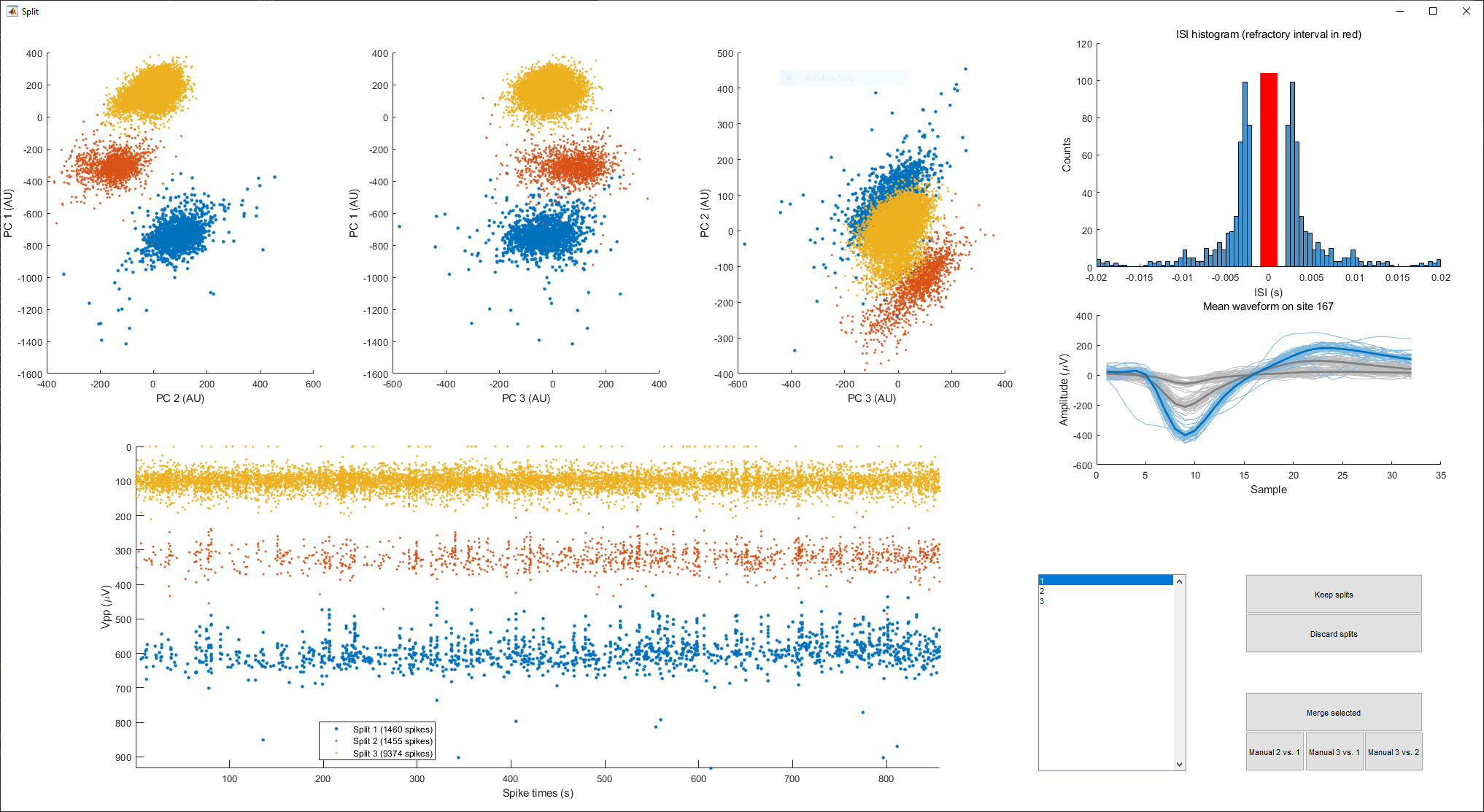
Two or more clusters may have been erroneously merged together by the algorithm. You can correct this by selecting the cluster in the waveform view and either pressing ‘s’ in the waveform view or selecting one of the Split options from the main menu. JRCLUST will then prompt you for the number of clusters you believe this cluster should be split into, and then perform hierarchical clustering on a set of features computed from the spikes in this cluster, using Ward’s minimum variance method . You may view projections of spikes onto the 1st, 2nd, and 3rd principal components, a μV peak-to-peak vs. time plot, an ISI histogram, and mean waveforms for each split or combination of splits. You may also choose to manually split in any of the PC spaces or merge splits together. When you are satisfied, you can select “Keep splits” and your cluster will be split If you change your mind you can select “Discard splits” and your cluster will be unaffected.

The similarity view (FigSim)

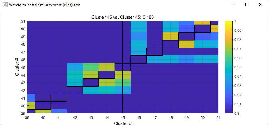
The similarity view tells you how similar each cluster is to every other. (Diagonal entries show self-similarity, lower-amplitude to higher-amplitude spikes.) Similarity is computed at clustering and every time the spike table changes. You may choose to automatically merge clusters whose similarity exceeds a given threshold (the default is 0.98) by selecting Merge auto from the Edit menu and supplying a different threshold. You may pan by holding the Shift key and clicking and dragging, or zoom in and out with the scroll wheel. The selected cluster is indicated by a crosshair at the center of a rectangle. To delete the selected cluster, press d. To split the selected cluster, press s. If two clusters are selected, then the crosshair will be red on the horizontal. To merge the selected pair of clusters, press m.

The feature-vs-time view (FigTime)

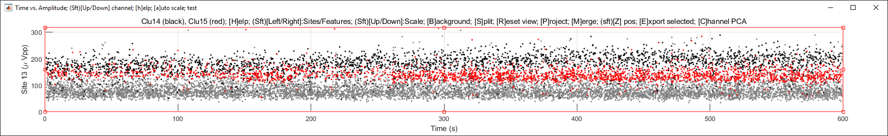
The feature-vs-time view displays a feature (by default the peak-to-peak amplitude (or Vpp), in μV) plotted against time (in seconds) on a given site. When selecting a unit, this feature is plotted on the center site of that unit, but you may change sites by pressing the left or right arrows, or adjust the scale with the up and down arrows. Press r to reset the view. The features shown for the selected cluster are in black, with background features in gray (toggle background features with the b key). If you select another cluster via the waveform or similarity views, features for the other cluster on that site will be shown in red. You can switch between the the Vpp and PCA by pressing f in this view. If two clusters are selected, you may merge them with m. If one cluster is selected, you may split it by pressing s and drawing a polygon around the points in the new cluster to split off.

The feature projection view (FigProj)

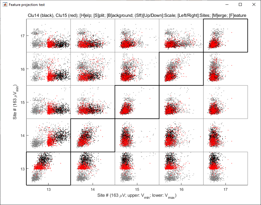
The feature projection view displays one feature vs. another on an adjacent group of sites. By default, these features are the minimum vs. maximum amplitudes on and below the diagonal, and minimum vs. minimum amplitudes above the diagonal. You may toggle the feature to display by pressing the f key, or by selecting one from the Projection menu. If showing the PCA feature, you may switch between PC2 vs. PC1, PC3 vs. PC1, or PC3 vs. PC2 with the p key. If two clusters are selected, you may merge them with m.

The ISI histogram view (FigHist)

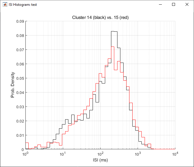
The ISI histogram shows a histogram of interspike intervals, i.e., intervals between firings (in ms) in the selected cluster.

The time correlation view (FigCorr)

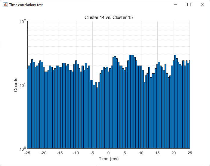
The time correlation view shows a count of spike firings at time lags of -25 ms to 25 ms, in 1/2 ms bins. If more than one cluster is selected, then the reference cluster is the primary selected cluster, and time lags are measured with respect to spikes in the reference cluster.

The return map view (FigISI)

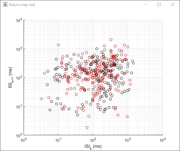
The return map view shows a sampling of interspike intervals (in milliseconds) from the selected cluster, plotted against the previous ISI. That is, if \(t_k\) denotes the length of the interval between spike \(k\) and spike \(k+1\), then this figure plots \(t_{k+1}\) vs. \(t_k\) for some subset of spikes in the selected cluster or clusters.

The probe map view (FigMap)

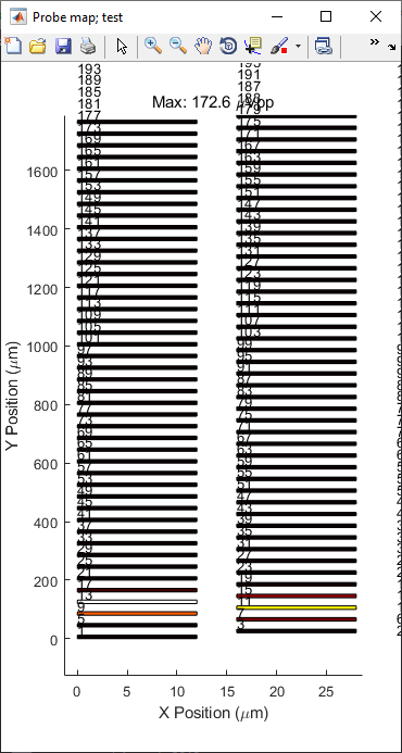
The probe map view plots a color-coded activity map on the probe site layout. The built-in hot color map is used to represent the Vpp of the average waveform of the selected cluster, so lighter colors indicate larger Vpp.

The probe position view (FigPos)

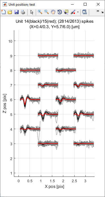
The probe position view shows the mean waveforms of the selected cluster or clusters on the probe. Whereas the waveform view shows the mean waveforms of each cluster stacked linearly, the position view shows where these waveforms are on the probe.

The rho-delta view (FigRD)

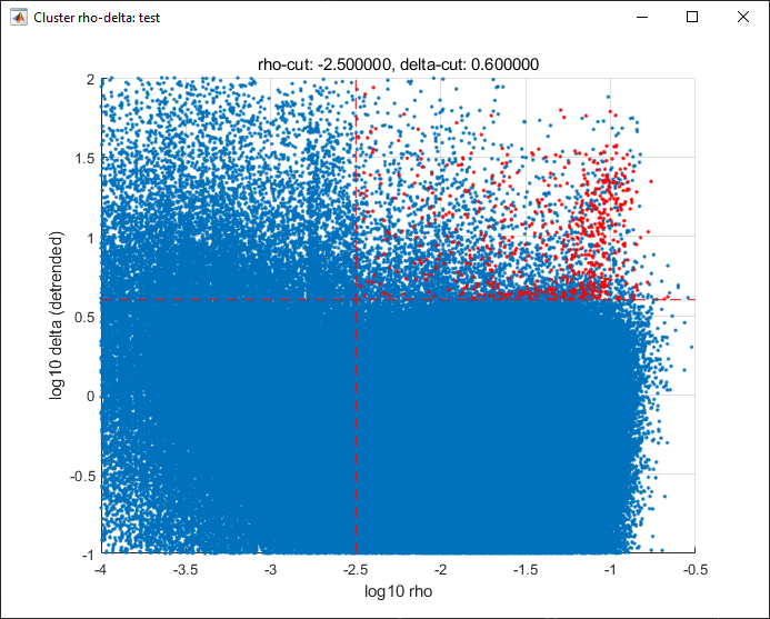
This figure shows the delta values plotted against the rho values for all spikes. Cluster centers are highlighted in red and the log10RhoCut and log10DeltaCut thresholds are plotted as dashed vertical and horizontal lines, respectively.