Spike clustering

Adjustments to the algorithm

Because many millions of spikes may be detected in a single recording and the distance matrix grows as \(O(n^2)\), we quickly run out of memory. Instead, we take advantage of the fact that two spikes which are far away from each other in space and in time are unlikely to be from the same neuron and thus should not belong to the same cluster. So instead of computing the distance between a spike and every other spike, we restrict our comparison of spikes on site \(K\) to spikes which either also peak on site \(K\), or have a secondary peak on site \(K\). Additionally, if you specify, we also restrict our comparison to spikes occurring nearby in time (you might want to do this if you observe drift in your recording). This has a tendency to oversplit clusters, but they can be merged later.

Determining \(d\)

The best cutoff distance in feature space is generally not known a priori. In order to determine a good cutoff distance, we instead estimate a percentile you specify (the 2nd percentile by default), call it \(d_i\), of the pairwise distances between spike features on each site \(i\). We then take the median of the \(d_i\) as our global cutoff distance.

(This behavior can be overridden by setting the parameter useGlobalDistCut to 0 in your config file.)

Assigning clusters: “sufficiently dense” and “sufficiently far”

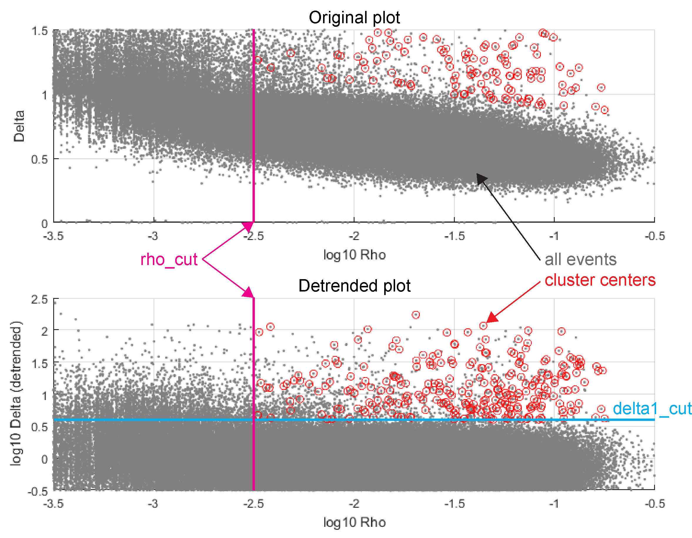
Once every spike has its \(\rho\) and \(\delta\) scores, along with the nearest neighbor of higher density corresponding to the \(\delta\) score, we then determine cluster centers.

You must specify the thresholds to determine a cluster center. In particular, a spike \(i\) must have \(\log_{10}(\rho_i) > \text{log10RhoCut}\) (“sufficiently dense”) and \(\log_{10}(\delta_i) > \text{log10DeltaCut}\) (“sufficiently far”). If you specify, this comparison may be made against a detrended plot, as in the images below.

Once cluster centers are assigned, it is a straightforward operation to assign spikes to clusters: for each spike which has not been assigned a cluster (initially, this is all spikes which are not cluster centers), assign it to the same cluster as its nearest neighbor of higher density. Most spikes will remain unassigned at first, but on each iteration of this procedure, the number of spikes which are unassigned will shrink until all spikes have been assigned to clusters.

Note

Because we compared primary peaks with secondary peaks, a spike may have as its nearest neighbor a spike on a nearby site.

Merging possibly oversplit clusters

After the initial clustering using, units with similar mean raw waveforms are merged based on their similarity, as computed using the Pearson correlation coefficient of the waveforms. Since probe drift changes the spike waveforms, averaged waveforms are computed at three depth ranges per unit using their center-of-mass positions. Additionally, a time shift is applied between each pair to find the maximum cross-correlation value. The similarity score is taken as the maximum score from the resulting \(3 \times 3\) correlation matrix for each unit pair. Any cluster pair whose maximum similarity exceeds a threshold you specify is merged.

This process is repeated some number of times and the resulting clustering is output for inspection.